8. Numpy와 PyTorch를 이용한 지하수 경로 예측(딥러닝, 지도학습)
데이터 전처리 및 학습 데이터 생성(Numpy)
import os
import json
import numpy as np
import pandas as pd
from shapely.geometry import LineString
import rasterio
from rasterio.transform import rowcol
from math import sqrt

# === 경로 설정 ===
BASE_DIR = os.path.dirname(os.path.abspath(__file__))
DATA_DIR = os.path.join(BASE_DIR, "data")
DEM_PATH = os.path.join(DATA_DIR, "DEM.tif")
GEOJSON_PATH = os.path.join(DATA_DIR, "지하수흐름.geojson")
OUTPUT_CSV = os.path.join(DATA_DIR, "flow_learning_dataset.csv")

# === DEM 열기 ===
with rasterio.open(DEM_PATH) as src:
    dem = src.read(1)
    transform = src.transform
    nodata = src.nodata

# NoData 마스킹
dem = np.ma.masked_equal(dem, nodata)

# === GeoJSON 로드 ===
with open(GEOJSON_PATH, "r", encoding="utf-8") as f:
    gj = json.load(f)

samples = []

# === 흐름선 따라 10m 간격 샘플링 ===
for feature in gj["features"]:
    coords_multi = feature["geometry"]["coordinates"]
    for coords in coords_multi:
        if len(coords) < 2:
            continue
        line = LineString(coords)
        for dist in np.arange(0, line.length, 10):  # 10m 간격
            pt = line.interpolate(dist)
            lon, lat = pt.x, pt.y
            try:
                row, col = rowcol(transform, lon, lat)
                if row < 1 or col < 1 or row + 2 > dem.shape[0] or col + 2 > dem.shape[1]:
                    continue
                kernel = dem[row-1:row+2, col-1:col+2]
                if np.ma.is_masked(kernel):
                    continue
                pt_next = line.interpolate(min(dist + 1, line.length))
                vx = pt_next.x - pt.x
                vy = pt_next.y - pt.y
                magnitude = sqrt(vx**2 + vy**2)
                if magnitude == 0:
                    continue
                vx /= magnitude
                vy /= magnitude
                samples.append((kernel.flatten().tolist(), [vx, vy]))
            except:
                continue

# === DataFrame 생성 및 저장 ===
X = [x for x, _ in samples]
y = [y for _, y in samples]
df_X = pd.DataFrame(X, columns=[f"elev_{i}" for i in range(9)])
df_y = pd.DataFrame(y, columns=["vx", "vy"])
df = pd.concat([df_X, df_y], axis=1)

df.to_csv(OUTPUT_CSV, index=False, encoding="utf-8-sig")
print(f"✅ 학습 데이터 저장 완료: {OUTPUT_CSV}")
print(f"총 샘플 수: {len(df)}")
DEM에 따라 어떤 지하수의 방향으로 흐르는지 각각의 위치에 따라 결과값(정답)을 구하고 그렇게 만들어진 데이터셋(flow_learning_dataset.csv)으로 다음 단계에서 학습모델을 만들 때 지도학습의 정답으로 사용할 것입니다.
elev_0,elev_1,elev_2,elev_3,elev_4,elev_5,elev_6,elev_7,elev_8,vx,vy
14.165233612060547,15.591638565063477,16.890029907226562,15.714686393737793,16.892200469970703,18.025903701782227,15.714686393737793,16.892200469970703,18.025903701782227,0.6141826252983711,-0.7891639264320187
162.5628662109375,155.6248321533203,141.26046752929688,166.32676696777344,161.97726440429688,145.39190673828125,210.35009765625,191.12039184570312,158.28128051757812,-0.9044362227904528,0.4266088593835559
320.59490966796875,320.59490966796875,287.78851318359375,312.6998291015625,312.6998291015625,276.14825439453125,299.16552734375,299.16552734375,264.07208251953125,-0.9623149989228065,-0.2719372038692004
47.63901901245117,53.15440368652344,53.15440368652344,48.99812698364258,56.309547424316406,56.309547424316406,59.914756774902344,61.57112503051758,61.57112503051758,-0.8853173882475284,0.46498722785316915
320.59490966796875,320.59490966796875,287.78851318359375,312.6998291015625,312.6998291015625,276.14825439453125,299.16552734375,299.16552734375,264.07208251953125,-0.8226409456566786,0.568561231996243
478.37286376953125,450.86407470703125,418.89862060546875,478.37286376953125,450.86407470703125,418.89862060546875,493.70318603515625,467.58685302734375,433.1954650878906,0.9886679545389438,-0.15011887179092767
이런 느낌으로 나옵니다. 간단히 설명하자면, elev_0,elev_1,elev_2,elev_3,elev_4,elev_5,elev_6,elev_7,elev_8은 3x3 커널(픽셀 블록) 내 고도 값. 중심점 기준 주변 8개를 포함한 고도 분포이고 vx,vy은 중심 픽셀에서 다음 위치까지의 단위 벡터 (지하수 흐름 방향)입니다.
모델 학습(PyTorch)
import os
import pandas as pd
import torch
import torch.nn as nn
from torch.utils.data import DataLoader, TensorDataset
from sklearn.model_selection import train_test_split

# ✅ 하이퍼파라미터
EPOCHS = 200
BATCH_SIZE = 64
LR = 0.001

# ✅ 현재 파일 기준으로 data 디렉토리 경로 만들기
BASE_DIR = os.path.dirname(os.path.abspath(__file__))  # 현재 .py 파일 경로
SAVE_DIR = os.path.join(BASE_DIR, "data")
MODEL_PATH = os.path.join(SAVE_DIR, "model.pth")

# ✅ 데이터 불러오기
csv_path = os.path.join(os.path.dirname(__file__), "data", "flow_learning_dataset.csv")
df = pd.read_csv(csv_path, encoding="utf-8-sig")  # <- 여기에 쉼표 ❌
X = df[[f"elev_{i}" for i in range(9)]].values
y = df[["vx", "vy"]].values

# ✅ train/test 분할
X_train, X_test, y_train, y_test = train_test_split(X, y, test_size=0.2, random_state=42)

# ✅ Tensor 변환
X_train = torch.FloatTensor(X_train)
y_train = torch.FloatTensor(y_train)
X_test = torch.FloatTensor(X_test)
y_test = torch.FloatTensor(y_test)

# ✅ DataLoader
train_loader = DataLoader(TensorDataset(X_train, y_train), batch_size=BATCH_SIZE, shuffle=True)
test_loader = DataLoader(TensorDataset(X_test, y_test), batch_size=BATCH_SIZE)

# ✅ MLP 모델 정의
class MLP(nn.Module):
    def __init__(self):
        super().__init__()
        self.net = nn.Sequential(
            nn.Linear(9, 64),
            nn.ReLU(),
            nn.Linear(64, 64),
            nn.ReLU(),
            nn.Linear(64, 2)  # vx, vy 출력
        )

    def forward(self, x):
        return self.net(x)

model = MLP()
criterion = nn.MSELoss()
optimizer = torch.optim.Adam(model.parameters(), lr=LR)

# ✅ 학습 루프
for epoch in range(EPOCHS):
    model.train()
    running_loss = 0.0
    for xb, yb in train_loader:
        pred = model(xb)
        loss = criterion(pred, yb)
        optimizer.zero_grad()
        loss.backward()
        optimizer.step()
        running_loss += loss.item()

    if (epoch + 1) % 10 == 0:
        print(f"Epoch {epoch+1}/{EPOCHS}, Loss: {running_loss/len(train_loader):.6f}")

# ✅ 모델 저장
torch.save(model.state_dict(), MODEL_PATH)
print("✅ 학습 완료 및 모델 저장: data/model.pth")
앞에서 전처리된 CSV 데이터(정답값)를 사용해, 고도 정보를 입력받아 지하수 흐름 방향 (vx, vy)을 예측하는 MLP(다층 퍼셉트론) 회귀 모델을 지도학습시키는 과정입니다. DEM의 고도 패턴과 흐름 방향 간 비선형 함수 근사를 시도하고자 했습니다. 그렇게 나온 모델이 바로 model.pth이고 이걸로 DEM 고도 값만 주면 학습된 모델을 통해 그 지점의 지하수 흐름(벡터)를 추론할 수 있습니다.
모델 추론 및 결과 저장(geojson)
import os
import torch
import geojson
import numpy as np
import pymysql
from math import sqrt
import rasterio
from rasterio.transform import rowcol
from shapely.geometry import LineString

# ✅ 경로 설정
BASE_DIR = os.path.dirname(os.path.abspath(__file__))
DEM_PATH = os.path.join(BASE_DIR, "data", "DEM.tif")
MODEL_PATH = os.path.join(BASE_DIR, "data", "model.pth")
OUTPUT_DIR = os.path.join(BASE_DIR, "..", "my-weather-map", "public", "data", "flow")
os.makedirs(OUTPUT_DIR, exist_ok=True)

# ✅ DEM 불러오기
with rasterio.open(DEM_PATH) as src:
    dem = src.read(1)
    transform = src.transform
    nodata = src.nodata

dem = np.ma.masked_equal(dem, nodata)

# ✅ MLP 모델 구조와 로드
class MLP(torch.nn.Module):
    def __init__(self):
        super().__init__()
        self.net = torch.nn.Sequential(
            torch.nn.Linear(9, 64),
            torch.nn.ReLU(),
            torch.nn.Linear(64, 64),
            torch.nn.ReLU(),
            torch.nn.Linear(64, 2)  # vx, vy
        )

    def forward(self, x):
        return self.net(x)

model = MLP()
model.load_state_dict(torch.load(MODEL_PATH, map_location="cpu"))
model.eval()

# ✅ 흐름 경로 예측 함수
def predict_path(start_lat, start_lng, max_steps=200, step_size=1.0):
    try:
        row, col = rowcol(transform, start_lng, start_lat)
    except:
        return []

    path = []

    for _ in range(max_steps):
        if (row < 1 or row + 2 >= dem.shape[0] or col < 1 or col + 2 >= dem.shape[1]):
            break

        kernel = dem[row-1:row+2, col-1:col+2]
        if np.ma.is_masked(kernel):
            break

        input_tensor = torch.FloatTensor(kernel.flatten()).unsqueeze(0)
        with torch.no_grad():
            vx, vy = model(input_tensor).squeeze().tolist()

        mag = sqrt(vx**2 + vy**2)
        if mag == 0:
            break

        # 이동
        row -= int(round((vy / mag) * step_size))
        col += int(round((vx / mag) * step_size))

        lng, lat = transform * (col, row)
        path.append((lat, lng))

    return path

# ✅ 오염원 DB에서 위치 불러오기
conn = pymysql.connect(
    host="www.lifeslike.org",
    user="water",
    password="water1111",
    database="weather_db",
    charset="utf8mb4",
    use_unicode=True
)
cursor = conn.cursor()
cursor.execute("SELECT id, latitude, longitude FROM pollution_sources WHERE latitude IS NOT NULL AND longitude IS NOT NULL")
rows = cursor.fetchall()

# ✅ 예측 및 저장
count = 0
for id, lat, lng in rows:
    path = predict_path(lat, lng)
    if len(path) < 2:
        continue

    feature = geojson.Feature(
        geometry=geojson.LineString([(lng_, lat_) for lat_, lng_ in path]),
        properties={"id": id}
    )
    geojson_obj = geojson.FeatureCollection([feature])

    out_path = os.path.join(OUTPUT_DIR, f"flow_path_{id}.geojson")
    with open(out_path, "w", encoding="utf-8") as f:
        geojson.dump(geojson_obj, f, ensure_ascii=False, indent=2)

    count += 1

print(f"✅ 예측된 흐름 경로 GeoJSON {count}개 생성 완료")
cursor.close()
conn.close()
학습된 모델(model.pth)을 활용하여 새로운 입력 데이터(원하는 위,경도)에 대한 예측을 수행하고, 그 결과를 시각화용 GeoJSON 파일로 저장합니다.
{
"type": "FeatureCollection",
"features": [
{
"type": "Feature",
"geometry": {
"type": "LineString",
"coordinates": [
[
127.978364,
37.307995
],
[
127.978364,
37.308803
],
[
127.978364,
37.309611
],
[
127.978364,
37.310419
],
[
127.977363,
37.311226
],
[
127.976362,
37.311226
],
[
127.976362,
37.312034
],
[
127.97536,
37.312034
],
[
127.97536,
37.312842
],
[
127.974359,
37.312842
],
[
127.974359,
37.31365
],
[
127.974359,
37.314458
],
[
127.974359,
37.315266
],
[
127.973357,
37.316074
],
[
127.973357,
37.316881
],
[
127.972356,
37.316881
],
[
127.972356,
37.317689
],
[
127.971354,
37.318497
],
[
127.970353,
37.319305
],
[
127.970353,
37.320113
],
[
127.970353,
37.320921
],
[
127.969352,
37.321728
],
[
127.96835,
37.321728
],
[
127.967349,
37.321728
],
[
127.967349,
37.322536
],
[
127.966347,
37.323344
],
[
127.966347,
37.324152
],
[
127.966347,
37.32496
],
[
127.966347,
37.325768
],
[
127.966347,
37.326576
],
[
127.965346,
37.327383
],
[
127.965346,
37.328191
],
[
127.965346,
37.328999
],
[
127.964345,
37.329807
],
[
127.964345,
37.330615
],
[
127.963343,
37.331423
],
[
127.962342,
37.332231
],
[
127.962342,
37.333038
],
[
127.962342,
37.333846
],
[
127.96134,
37.334654
],
[
127.96134,
37.335462
],
[
127.96134,
37.33627
],
[
127.96134,
37.337078
],
[
127.96134,
37.337886
],
[
127.96134,
37.338693
],
[
127.96134,
37.339501
],
[
127.96134,
37.340309
],
[
127.96134,
37.341117
],
[
127.96134,
37.341925
],
[
127.96134,
37.342733
],
[
127.96134,
37.343541
],
[
127.962342,
37.344348
],
[
127.96134,
37.345156
],
[
127.960339,
37.345156
],
[
127.960339,
37.345964
],
[
127.959337,
37.345964
],
[
127.958336,
37.346772
],
[
127.958336,
37.34758
],
[
127.957335,
37.348388
],
[
127.956333,
37.349196
],
[
127.955332,
37.349196
],
[
127.95433,
37.350003
],
[
127.95433,
37.350811
],
[
127.953329,
37.351619
],
[
127.953329,
37.352427
],
[
127.953329,
37.353235
],
[
127.952328,
37.354043
],
[
127.952328,
37.35485
],
[
127.952328,
37.355658
],
[
127.952328,
37.356466
],
[
127.952328,
37.357274
],
[
127.952328,
37.358082
],
[
127.951326,
37.35889
],
[
127.951326,
37.359698
],
[
127.951326,
37.360505
],
[
127.951326,
37.361313
],
[
127.951326,
37.362121
],
[
127.950325,
37.362929
],
[
127.950325,
37.363737
],
[
127.949323,
37.363737
],
[
127.950325,
37.364545
],
[
127.949323,
37.364545
],
[
127.949323,
37.365353
],
[
127.949323,
37.36616
],
[
127.948322,
37.366968
],
[
127.948322,
37.367776
],
[
127.948322,
37.368584
],
[
127.948322,
37.369392
],
[
127.948322,
37.3702
],
[
127.94732,
37.369392
],
[
127.94732,
37.3702
],
[
127.946319,
37.3702
],
[
127.946319,
37.371008
],
[
127.946319,
37.371815
],
[
127.946319,
37.372623
],
[
127.946319,
37.373431
],
[
127.946319,
37.374239
],
[
127.946319,
37.375047
],
[
127.946319,
37.375855
],
[
127.946319,
37.376663
],
[
127.946319,
37.37747
],
[
127.946319,
37.378278
],
[
127.946319,
37.379086
],
[
127.946319,
37.379894
],
[
127.946319,
37.380702
],
[
127.946319,
37.38151
],
[
127.946319,
37.382317
],
[
127.946319,
37.383125
],
[
127.945318,
37.383933
],
[
127.944316,
37.384741
],
[
127.944316,
37.385549
],
[
127.944316,
37.386357
],
[
127.944316,
37.387165
],
[
127.944316,
37.387972
],
[
127.943315,
37.38878
],
[
127.942313,
37.38878
],
[
127.941312,
37.389588
],
[
127.941312,
37.390396
],
[
127.940311,
37.390396
],
[
127.940311,
37.391204
],
[
127.940311,
37.392012
],
[
127.939309,
37.392012
],
[
127.939309,
37.39282
],
[
127.938308,
37.393627
],
[
127.937306,
37.394435
],
[
127.937306,
37.395243
],
[
127.937306,
37.396051
],
[
127.936305,
37.396051
],
[
127.936305,
37.396859
],
[
127.935303,
37.396859
],
[
127.935303,
37.397667
],
[
127.934302,
37.398475
],
[
127.933301,
37.399282
],
[
127.933301,
37.40009
],
[
127.933301,
37.400898
],
[
127.932299,
37.401706
],
[
127.932299,
37.402514
],
[
127.931298,
37.403322
],
[
127.931298,
37.40413
],
[
127.930296,
37.404937
],
[
127.929295,
37.405745
],
[
127.928294,
37.404937
],
[
127.928294,
37.405745
],
[
127.928294,
37.406553
],
[
127.927292,
37.407361
],
[
127.928294,
37.408169
],
[
127.927292,
37.408169
],
[
127.926291,
37.408169
],
[
127.926291,
37.408977
],
[
127.926291,
37.409785
],
[
127.925289,
37.410592
],
[
127.924288,
37.4114
],
[
127.923286,
37.4114
],
[
127.924288,
37.4114
],
[
127.923286,
37.4114
],
[
127.924288,
37.4114
],
[
127.923286,
37.4114
],
[
127.924288,
37.4114
],
[
127.923286,
37.4114
],
[
127.924288,
37.4114
],
[
127.923286,
37.4114
],
[
127.924288,
37.4114
],
[
127.923286,
37.4114
],
[
127.924288,
37.4114
],
[
127.923286,
37.4114
],
[
127.924288,
37.4114
],
[
127.923286,
37.4114
],
[
127.924288,
37.4114
],
[
127.923286,
37.4114
],
[
127.924288,
37.4114
],
[
127.923286,
37.4114
],
[
127.924288,
37.4114
],
[
127.923286,
37.4114
],
[
127.924288,
37.4114
],
[
127.923286,
37.4114
],
[
127.924288,
37.4114
],
[
127.923286,
37.4114
],
[
127.924288,
37.4114
],
[
127.923286,
37.4114
],
[
127.924288,
37.4114
],
[
127.923286,
37.4114
],
[
127.924288,
37.4114
],
[
127.923286,
37.4114
],
[
127.924288,
37.4114
],
[
127.923286,
37.4114
],
[
127.924288,
37.4114
],
[
127.923286,
37.4114
],
[
127.924288,
37.4114
],
[
127.923286,
37.4114
],
[
127.924288,
37.4114
],
[
127.923286,
37.4114
],
[
127.924288,
37.4114
],
[
127.923286,
37.4114
],
[
127.924288,
37.4114
],
[
127.923286,
37.4114
],
[
127.924288,
37.4114
],
[
127.923286,
37.4114
],
[
127.924288,
37.4114
],
[
127.923286,
37.4114
],
[
127.924288,
37.4114
]
]
},
"properties": {
"id": 1
}
}
]
}
하나만 예시로 보여드리면 이렇게 추론 결과가 geojson형태로 나오고 이걸 LineString형태로 맵에 표시해주면 됩니다.
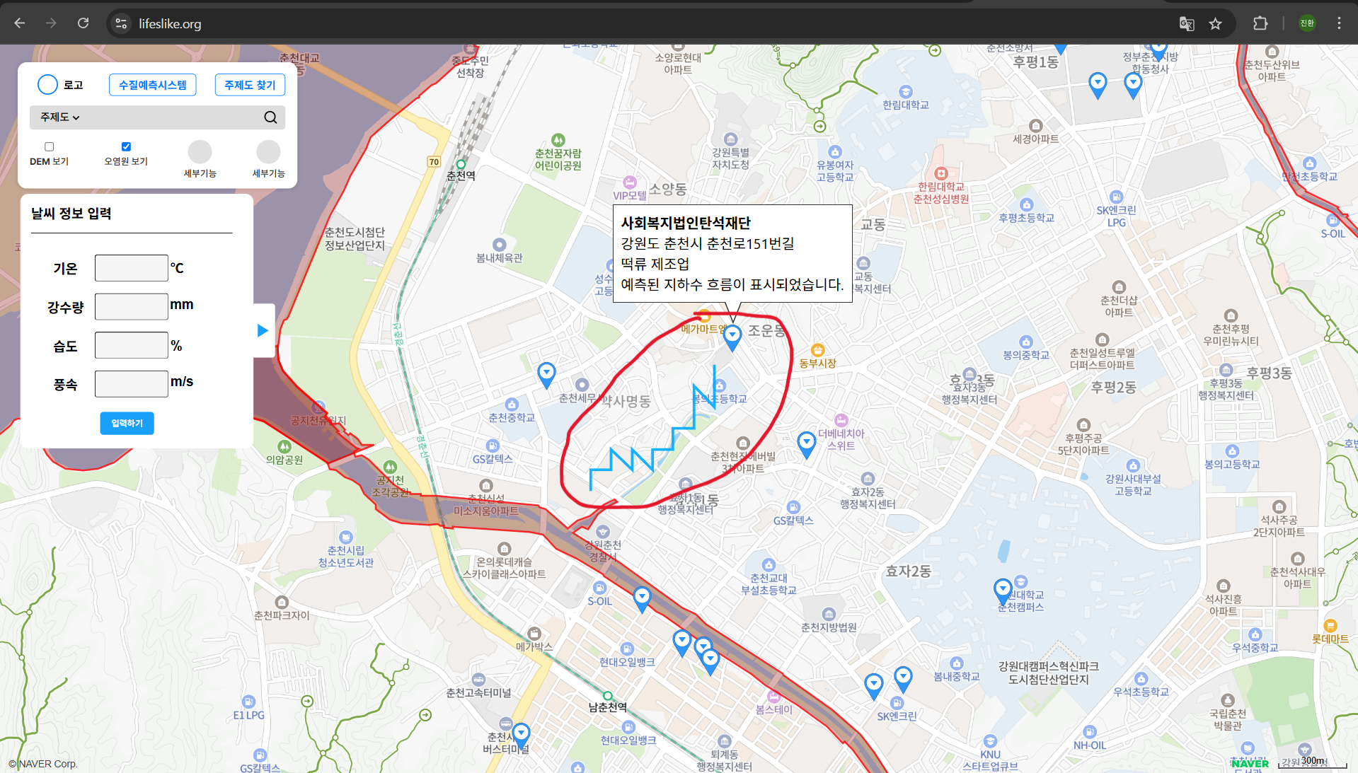
실제 적용한 화면입니다.